Plot to compare estimates from original and follow-up studies
Source:R/meta_plots.R
replicate.plot.RdGenerates a basic plot using ggplot2 to visualize the estimates from the original and follow-up studies.
Usage
replicate.plot(
  result,
  focus = c("Both", "Difference", "Average"),
  reference_line = NULL,
  diamond_height = 0.2,
  difference_axis_ticks = 5,
  ggtheme = ggplot2::theme_classic()
)
Arguments
- result
a result matrix from any of the replicate functions in vcmeta
- focus
Optional specification of the focus of the plot; defaults to 'Both'
Both - plots each estimate, difference, and average
Difference - plot each estimate and difference between them
Average - plot each estimate and the average effect size
- reference_line
Optional x-value for a reference line. Only applies if focus is 'Difference' or 'Both'. Defaults to NULL, in which case a reference line is not drawn.
- diamond_height
Optional height of the diamond representing average effect size. Only applies if focus is 'Average' or 'Both'. Defaults to 0.2
- difference_axis_ticks
Optional requested number of ticks on the difference axis. Only applies if focus is 'Difference' or 'Both'. Defaults to 5.
- ggtheme
optional ggplot2 theme object; defaults to theme_classic()
Examples
# Compare Damisch et al., 2010 to Calin-Jageman & Caldwell 2014
# Damisch et al., 2010, Exp 1, German participants made 10 mini-golf putts.
# Half were told they had a 'lucky' golf ball; half were not.
# Found a large but uncertain improvement in shots made in the luck condition
# Calin-Jageman & Caldwell, 2014, Exp 1, was a pre-registered replication with
# input from Damisch, though with English-speaking participants.
#
# Here we compare the effect sizes, in original units, for the two studies.
# Use the replicate.mean2 function because the design is a 2-group design.
library(ggplot2)
damisch_v_calinjageman_raw <- replicate.mean2(
alpha = 0.05,
m11 = 6.42,
m12 = 4.75,
sd11 = 1.88,
sd12 = 2.15,
n11 = 14,
n12 = 14,
m21 = 4.73,
m22 = 4.62,
sd21 = 1.958,
sd22 = 2.12,
n21 = 66,
n22 = 58
)
# View the comparison:
damisch_v_calinjageman_raw
#> Estimate SE t p LL UL
#> Original: 1.67 0.7633058 2.188 0.038 0.09964253 3.2403575
#> Follow-up: 0.11 0.3682078 0.299 0.766 -0.61922358 0.8392236
#> Original - Follow-up: 1.56 0.8474743 1.841 0.073 0.13153488 2.9884651
#> Average: 0.89 0.4237372 2.100 0.042 0.03245567 1.7475443
#> df
#> Original: 25.55
#> Follow-up: 116.89
#> Original - Follow-up: 38.36
#> Average: 38.36
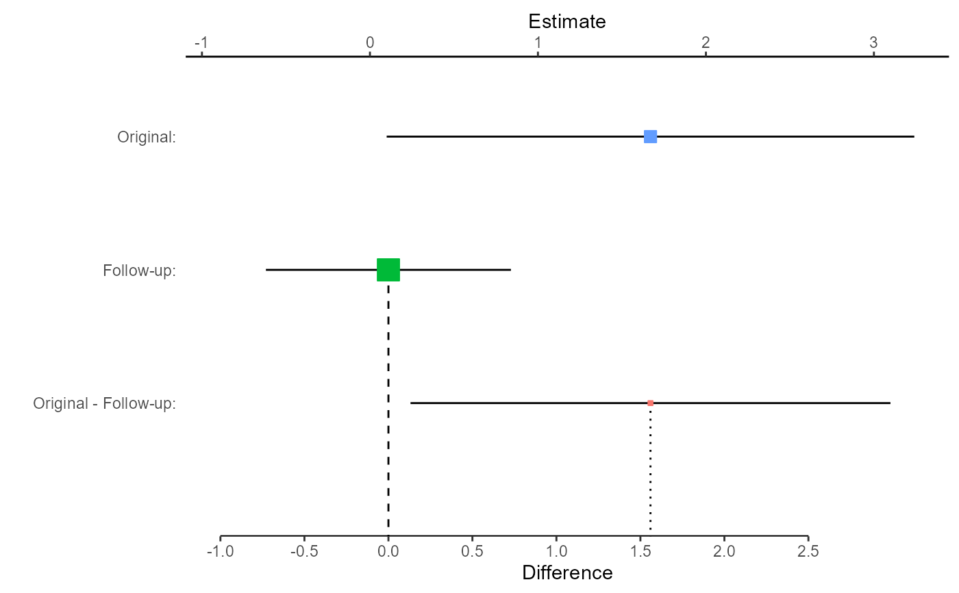
# Now plot the comparison, focusing on the difference
replicate.plot(damisch_v_calinjageman_raw, focus = "Difference")
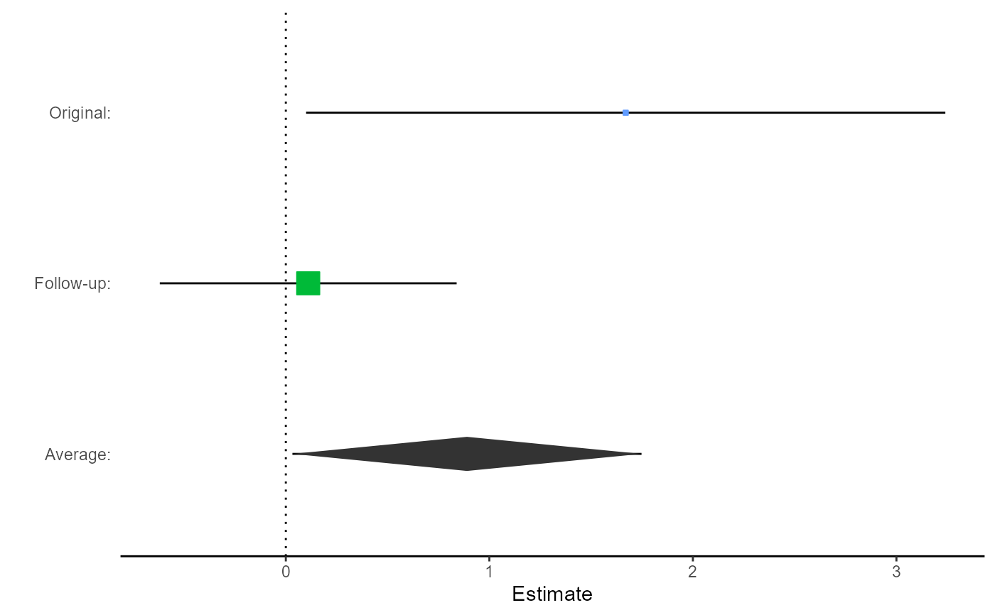
 # Plot the comparison, focusing on the average
replicate.plot(damisch_v_calinjageman_raw,
focus = "Average",
reference_line = 0,
diamond_height = 0.1
)
# Plot the comparison, focusing on the average
replicate.plot(damisch_v_calinjageman_raw,
focus = "Average",
reference_line = 0,
diamond_height = 0.1
)
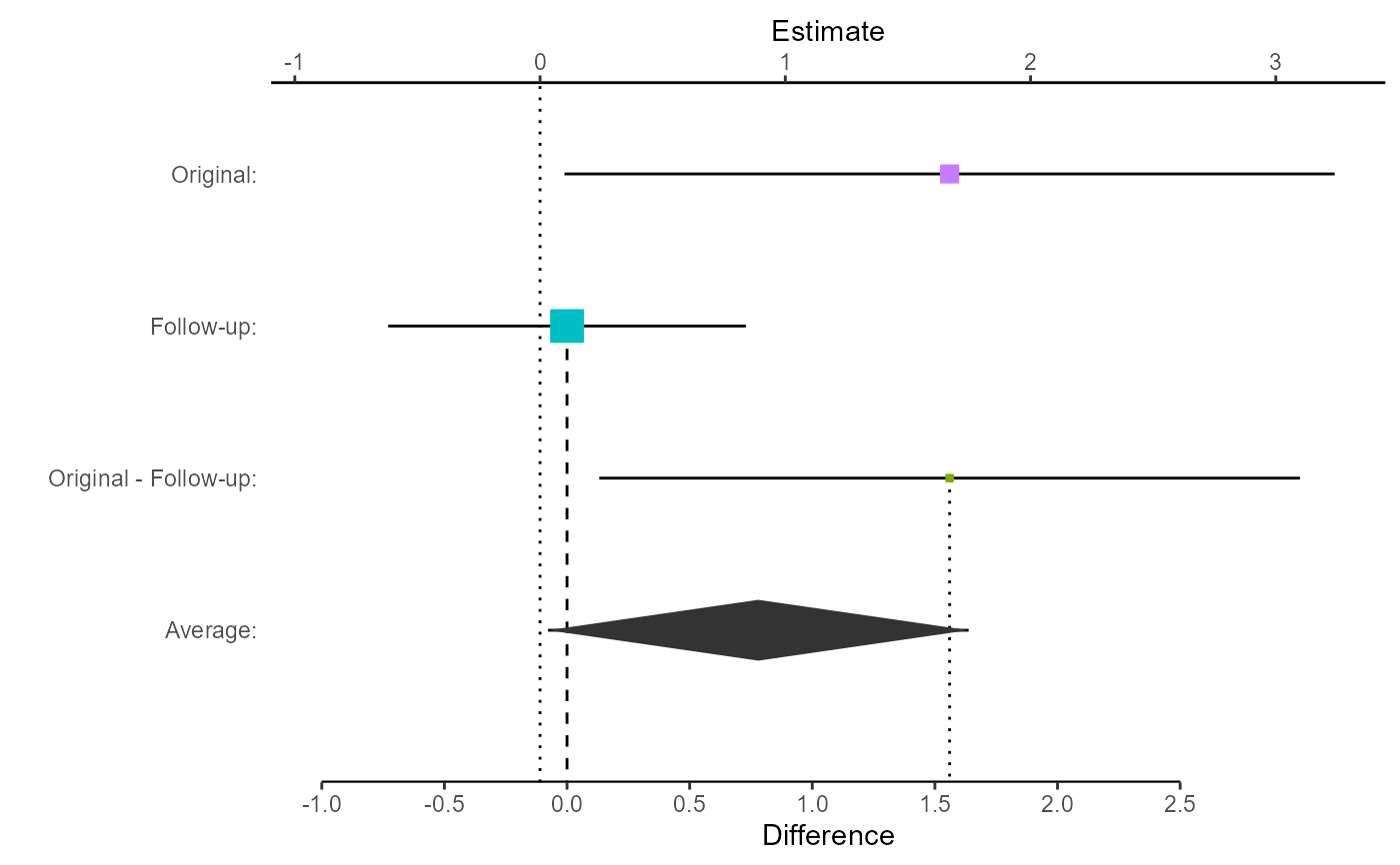
 # Plot the comparison with both difference and average.
# In this case, store the plot for manipulation
myplot <- replicate.plot(
damisch_v_calinjageman_raw,
focus = "Both",
reference_line = 0
)
# View the stored plot
myplot
# Plot the comparison with both difference and average.
# In this case, store the plot for manipulation
myplot <- replicate.plot(
damisch_v_calinjageman_raw,
focus = "Both",
reference_line = 0
)
# View the stored plot
myplot
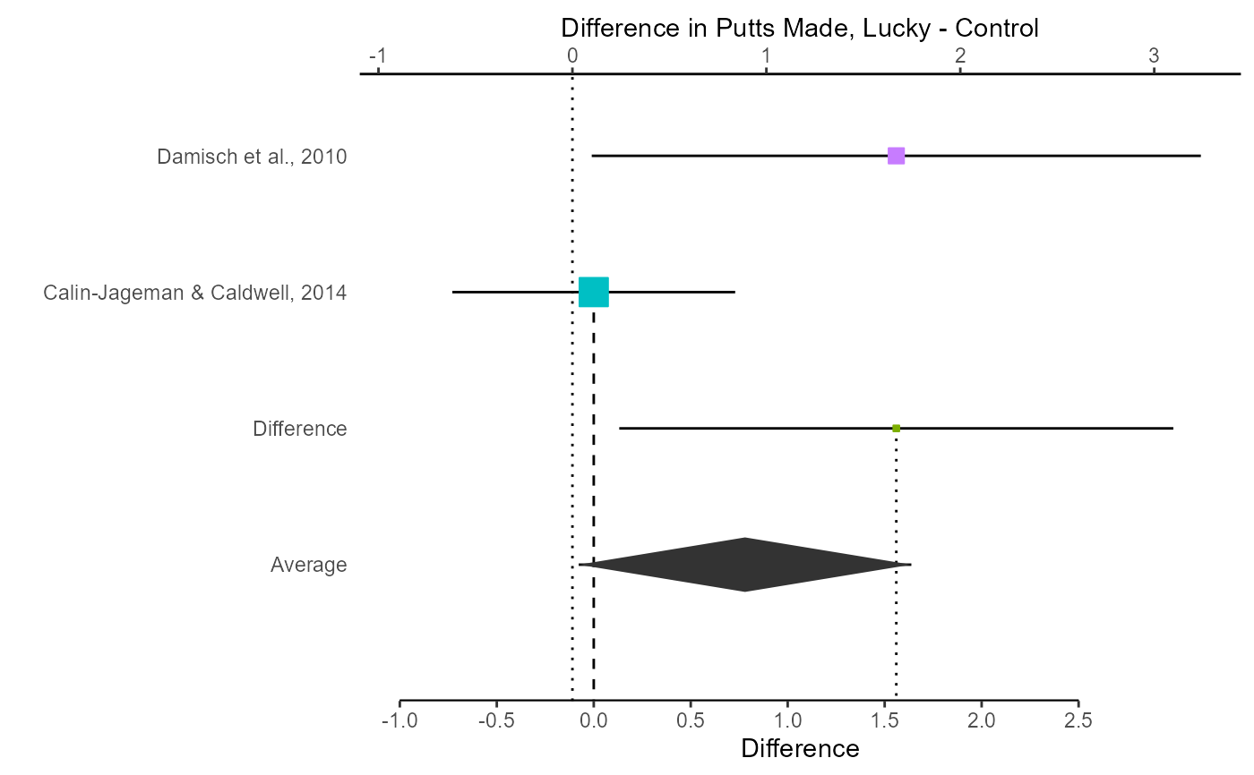
 # Change x-labels and study labels
myplot <- myplot + xlab("Difference in Putts Made, Lucky - Control")
myplot <- myplot + scale_y_discrete(
labels = c(
"Average",
"Difference",
"Calin-Jageman & Caldwell, 2014",
"Damisch et al., 2010"
)
)
# View the updated plot
myplot
# Change x-labels and study labels
myplot <- myplot + xlab("Difference in Putts Made, Lucky - Control")
myplot <- myplot + scale_y_discrete(
labels = c(
"Average",
"Difference",
"Calin-Jageman & Caldwell, 2014",
"Damisch et al., 2010"
)
)
# View the updated plot
myplot